Marketing Data
Data Marketing Analysis from Kaggle
Section 01: Exploratory Data Analysis
Let’s analyze the marketing data set provided by an user of Kaggle.
setwd("C:/Users/Daniel Gutierrez/Desktop/R Practice/Marketing Data Kaggle")
marketing_data <- readr::read_csv("marketing_data.csv")
Simple summary statistics of the data sets to see what variables we have
summary(marketing_data)## ID Year_Birth Education Marital_Status
## Min. : 0 Min. :1893 Length:2240 Length:2240
## 1st Qu.: 2828 1st Qu.:1959 Class :character Class :character
## Median : 5458 Median :1970 Mode :character Mode :character
## Mean : 5592 Mean :1969
## 3rd Qu.: 8428 3rd Qu.:1977
## Max. :11191 Max. :1996
## Income Kidhome Teenhome Dt_Customer
## Length:2240 Min. :0.0000 Min. :0.0000 Length:2240
## Class :character 1st Qu.:0.0000 1st Qu.:0.0000 Class :character
## Mode :character Median :0.0000 Median :0.0000 Mode :character
## Mean :0.4442 Mean :0.5062
## 3rd Qu.:1.0000 3rd Qu.:1.0000
## Max. :2.0000 Max. :2.0000
## Recency MntWines MntFruits MntMeatProducts
## Min. : 0.00 Min. : 0.00 Min. : 0.0 Min. : 0.0
## 1st Qu.:24.00 1st Qu.: 23.75 1st Qu.: 1.0 1st Qu.: 16.0
## Median :49.00 Median : 173.50 Median : 8.0 Median : 67.0
## Mean :49.11 Mean : 303.94 Mean : 26.3 Mean : 166.9
## 3rd Qu.:74.00 3rd Qu.: 504.25 3rd Qu.: 33.0 3rd Qu.: 232.0
## Max. :99.00 Max. :1493.00 Max. :199.0 Max. :1725.0
## MntFishProducts MntSweetProducts MntGoldProds NumDealsPurchases
## Min. : 0.00 Min. : 0.00 Min. : 0.00 Min. : 0.000
## 1st Qu.: 3.00 1st Qu.: 1.00 1st Qu.: 9.00 1st Qu.: 1.000
## Median : 12.00 Median : 8.00 Median : 24.00 Median : 2.000
## Mean : 37.53 Mean : 27.06 Mean : 44.02 Mean : 2.325
## 3rd Qu.: 50.00 3rd Qu.: 33.00 3rd Qu.: 56.00 3rd Qu.: 3.000
## Max. :259.00 Max. :263.00 Max. :362.00 Max. :15.000
## NumWebPurchases NumCatalogPurchases NumStorePurchases NumWebVisitsMonth
## Min. : 0.000 Min. : 0.000 Min. : 0.00 Min. : 0.000
## 1st Qu.: 2.000 1st Qu.: 0.000 1st Qu.: 3.00 1st Qu.: 3.000
## Median : 4.000 Median : 2.000 Median : 5.00 Median : 6.000
## Mean : 4.085 Mean : 2.662 Mean : 5.79 Mean : 5.317
## 3rd Qu.: 6.000 3rd Qu.: 4.000 3rd Qu.: 8.00 3rd Qu.: 7.000
## Max. :27.000 Max. :28.000 Max. :13.00 Max. :20.000
## AcceptedCmp3 AcceptedCmp4 AcceptedCmp5 AcceptedCmp1
## Min. :0.00000 Min. :0.00000 Min. :0.00000 Min. :0.00000
## 1st Qu.:0.00000 1st Qu.:0.00000 1st Qu.:0.00000 1st Qu.:0.00000
## Median :0.00000 Median :0.00000 Median :0.00000 Median :0.00000
## Mean :0.07277 Mean :0.07455 Mean :0.07277 Mean :0.06429
## 3rd Qu.:0.00000 3rd Qu.:0.00000 3rd Qu.:0.00000 3rd Qu.:0.00000
## Max. :1.00000 Max. :1.00000 Max. :1.00000 Max. :1.00000
## AcceptedCmp2 Response Complain Country
## Min. :0.00000 Min. :0.0000 Min. :0.000000 Length:2240
## 1st Qu.:0.00000 1st Qu.:0.0000 1st Qu.:0.000000 Class :character
## Median :0.00000 Median :0.0000 Median :0.000000 Mode :character
## Mean :0.01339 Mean :0.1491 Mean :0.009375
## 3rd Qu.:0.00000 3rd Qu.:0.0000 3rd Qu.:0.000000
## Max. :1.00000 Max. :1.0000 Max. :1.000000str(marketing_data)## spec_tbl_df [2,240 x 28] (S3: spec_tbl_df/tbl_df/tbl/data.frame)
## $ ID : num [1:2240] 1826 1 10476 1386 5371 ...
## $ Year_Birth : num [1:2240] 1970 1961 1958 1967 1989 ...
## $ Education : chr [1:2240] "Graduation" "Graduation" "Graduation" "Graduation" ...
## $ Marital_Status : chr [1:2240] "Divorced" "Single" "Married" "Together" ...
## $ Income : chr [1:2240] "$84,835.00" "$57,091.00" "$67,267.00" "$32,474.00" ...
## $ Kidhome : num [1:2240] 0 0 0 1 1 0 0 0 0 0 ...
## $ Teenhome : num [1:2240] 0 0 1 1 0 0 0 1 1 1 ...
## $ Dt_Customer : chr [1:2240] "6/16/14" "6/15/14" "5/13/14" "5/11/14" ...
## $ Recency : num [1:2240] 0 0 0 0 0 0 0 0 0 0 ...
## $ MntWines : num [1:2240] 189 464 134 10 6 336 769 78 384 384 ...
## $ MntFruits : num [1:2240] 104 5 11 0 16 130 80 0 0 0 ...
## $ MntMeatProducts : num [1:2240] 379 64 59 1 24 411 252 11 102 102 ...
## $ MntFishProducts : num [1:2240] 111 7 15 0 11 240 15 0 21 21 ...
## $ MntSweetProducts : num [1:2240] 189 0 2 0 0 32 34 0 32 32 ...
## $ MntGoldProds : num [1:2240] 218 37 30 0 34 43 65 7 5 5 ...
## $ NumDealsPurchases : num [1:2240] 1 1 1 1 2 1 1 1 3 3 ...
## $ NumWebPurchases : num [1:2240] 4 7 3 1 3 4 10 2 6 6 ...
## $ NumCatalogPurchases: num [1:2240] 4 3 2 0 1 7 10 1 2 2 ...
## $ NumStorePurchases : num [1:2240] 6 7 5 2 2 5 7 3 9 9 ...
## $ NumWebVisitsMonth : num [1:2240] 1 5 2 7 7 2 6 5 4 4 ...
## $ AcceptedCmp3 : num [1:2240] 0 0 0 0 1 0 1 0 0 0 ...
## $ AcceptedCmp4 : num [1:2240] 0 0 0 0 0 0 0 0 0 0 ...
## $ AcceptedCmp5 : num [1:2240] 0 0 0 0 0 0 0 0 0 0 ...
## $ AcceptedCmp1 : num [1:2240] 0 0 0 0 0 0 0 0 0 0 ...
## $ AcceptedCmp2 : num [1:2240] 0 1 0 0 0 0 0 0 0 0 ...
## $ Response : num [1:2240] 1 1 0 0 1 1 1 0 0 0 ...
## $ Complain : num [1:2240] 0 0 0 0 0 0 0 0 0 0 ...
## $ Country : chr [1:2240] "SP" "CA" "US" "AUS" ...
## - attr(*, "spec")=
## .. cols(
## .. ID = col_double(),
## .. Year_Birth = col_double(),
## .. Education = col_character(),
## .. Marital_Status = col_character(),
## .. Income = col_character(),
## .. Kidhome = col_double(),
## .. Teenhome = col_double(),
## .. Dt_Customer = col_character(),
## .. Recency = col_double(),
## .. MntWines = col_double(),
## .. MntFruits = col_double(),
## .. MntMeatProducts = col_double(),
## .. MntFishProducts = col_double(),
## .. MntSweetProducts = col_double(),
## .. MntGoldProds = col_double(),
## .. NumDealsPurchases = col_double(),
## .. NumWebPurchases = col_double(),
## .. NumCatalogPurchases = col_double(),
## .. NumStorePurchases = col_double(),
## .. NumWebVisitsMonth = col_double(),
## .. AcceptedCmp3 = col_double(),
## .. AcceptedCmp4 = col_double(),
## .. AcceptedCmp5 = col_double(),
## .. AcceptedCmp1 = col_double(),
## .. AcceptedCmp2 = col_double(),
## .. Response = col_double(),
## .. Complain = col_double(),
## .. Country = col_character()
## .. )
## - attr(*, "problems")=<externalptr>ID: Customer’s unique identifier
Year_Birth: Customer’s birth year
Education: Customer’s education level
Marital_Status: Customer’s marital status
Income: Customer’s yearly household income
Kidhome: Number of children in customer’s household
Teenhome: Number of teenagers in customer’s household
Dt_Customer: Date of customer’s enrollment with the company
Recency: Number of days since customer’s last purchase
MntWines: Amount spent on wine in the last 2 years
MntFruits: Amount spent on wine in the last 2 years
MntMeatProducts: Amount spent on meat in the last 2 years
MntFishProducts: Amount spent on fish in the last 2 years
MntSweetProducts: Amount spent on sweets in the last 2 years
MntGoldProds: Amount spent on gold in the last 2 years
NumDealsPurchase: Number of purchases made with a discount
NumWebPurchases: Number of purchases made through the company’s web site
NumCatalogPurchases: Number of purchases made using a catalogue
NumStorePurchases: Number of purchases made directly in stores
NumWebVisitsMonth: Number of visits to company’s web site in the last month
AcceptedCmp3: 1 if customer accepted the offer in the 3rd campaign, 0 otherwise
AcceptedCmp4: 1 if customer accepted the offer in the 4th campaign, 0 otherwise
AcceptedCmp5: 1 if customer accepted the offer in the 5th campaign, 0 otherwise
AcceptedCmp1: 1 if customer accepted the offer in the 1st campaign, 0 otherwise
AcceptedCmp2: 1 if customer accepted the offer in the 2nd campaign, 0 otherwise
Response: 1 if customer accepted the offer in the last campaign, 0 otherwise
Complain: 1 if customer complained in the last 2 years, 0 otherwise
Country: Customer’s location
Note that we have a variable, “year_birth”, for the costumers which probably is hard to interpret in a model. We would have to build an age variable. Also, note that the income variable is a string variable. It includes the dollar symbol, “$”, before the yearly income. Dt_Customer is a supposed to be a date.
We have to transform the income variable into a numerical variable. Marital status, education, accepted* and response as factors. Maybe country as a factor too. Also an age variable: 2021 - year_birth.
marketing <- marketing_data %>%
  mutate(Income = as.numeric(gsub("[^0-9.-]", "",Income)),
         Dt_Customer = as.Date(Dt_Customer, "%m/%d/%y"),
         Education = as.factor(Education),
         Marital_Status = as.factor(Marital_Status),
         Country = as.factor(Country),
         AcceptedCmp1 = as.factor(AcceptedCmp1),
         AcceptedCmp2 = as.factor(AcceptedCmp2),
         AcceptedCmp3 = as.factor(AcceptedCmp3),
         AcceptedCmp4 = as.factor(AcceptedCmp4),
         AcceptedCmp5 = as.factor(AcceptedCmp5),
         Response = as.factor(Response),
         Age = 2021 - Year_Birth)
marketing
## # A tibble: 2,240 x 29
## ID Year_Birth Education Marital_Status Income Kidhome Teenhome Dt_Customer
## <dbl> <dbl> <fct> <fct> <dbl> <dbl> <dbl> <date>
## 1 1826 1970 Graduation Divorced 84835 0 0 2014-06-16
## 2 1 1961 Graduation Single 57091 0 0 2014-06-15
## 3 10476 1958 Graduation Married 67267 0 1 2014-05-13
## 4 1386 1967 Graduation Together 32474 1 1 2014-05-11
## 5 5371 1989 Graduation Single 21474 1 0 2014-04-08
## 6 7348 1958 PhD Single 71691 0 0 2014-03-17
## 7 4073 1954 2n Cycle Married 63564 0 0 2014-01-29
## 8 1991 1967 Graduation Together 44931 0 1 2014-01-18
## 9 4047 1954 PhD Married 65324 0 1 2014-01-11
## 10 9477 1954 PhD Married 65324 0 1 2014-01-11
## # ... with 2,230 more rows, and 21 more variables: Recency <dbl>,
## # MntWines <dbl>, MntFruits <dbl>, MntMeatProducts <dbl>,
## # MntFishProducts <dbl>, MntSweetProducts <dbl>, MntGoldProds <dbl>,
## # NumDealsPurchases <dbl>, NumWebPurchases <dbl>, NumCatalogPurchases <dbl>,
## # NumStorePurchases <dbl>, NumWebVisitsMonth <dbl>, AcceptedCmp3 <fct>,
## # AcceptedCmp4 <fct>, AcceptedCmp5 <fct>, AcceptedCmp1 <fct>,
## # AcceptedCmp2 <fct>, Response <fct>, Complain <dbl>, Country <fct>, ...The raw the data set now looks better. But there are some NA’s. Let’s investigate them.
summary(marketing)## ID Year_Birth Education Marital_Status
## Min. : 0 Min. :1893 2n Cycle : 203 Married :864
## 1st Qu.: 2828 1st Qu.:1959 Basic : 54 Together:580
## Median : 5458 Median :1970 Graduation:1127 Single :480
## Mean : 5592 Mean :1969 Master : 370 Divorced:232
## 3rd Qu.: 8428 3rd Qu.:1977 PhD : 486 Widow : 77
## Max. :11191 Max. :1996 Alone : 3
## (Other) : 4
## Income Kidhome Teenhome Dt_Customer
## Min. : 1730 Min. :0.0000 Min. :0.0000 Min. :2012-07-30
## 1st Qu.: 35303 1st Qu.:0.0000 1st Qu.:0.0000 1st Qu.:2013-01-16
## Median : 51382 Median :0.0000 Median :0.0000 Median :2013-07-08
## Mean : 52247 Mean :0.4442 Mean :0.5062 Mean :2013-07-10
## 3rd Qu.: 68522 3rd Qu.:1.0000 3rd Qu.:1.0000 3rd Qu.:2013-12-30
## Max. :666666 Max. :2.0000 Max. :2.0000 Max. :2014-06-29
## NA's :24
## Recency MntWines MntFruits MntMeatProducts
## Min. : 0.00 Min. : 0.00 Min. : 0.0 Min. : 0.0
## 1st Qu.:24.00 1st Qu.: 23.75 1st Qu.: 1.0 1st Qu.: 16.0
## Median :49.00 Median : 173.50 Median : 8.0 Median : 67.0
## Mean :49.11 Mean : 303.94 Mean : 26.3 Mean : 166.9
## 3rd Qu.:74.00 3rd Qu.: 504.25 3rd Qu.: 33.0 3rd Qu.: 232.0
## Max. :99.00 Max. :1493.00 Max. :199.0 Max. :1725.0
##
## MntFishProducts MntSweetProducts MntGoldProds NumDealsPurchases
## Min. : 0.00 Min. : 0.00 Min. : 0.00 Min. : 0.000
## 1st Qu.: 3.00 1st Qu.: 1.00 1st Qu.: 9.00 1st Qu.: 1.000
## Median : 12.00 Median : 8.00 Median : 24.00 Median : 2.000
## Mean : 37.53 Mean : 27.06 Mean : 44.02 Mean : 2.325
## 3rd Qu.: 50.00 3rd Qu.: 33.00 3rd Qu.: 56.00 3rd Qu.: 3.000
## Max. :259.00 Max. :263.00 Max. :362.00 Max. :15.000
##
## NumWebPurchases NumCatalogPurchases NumStorePurchases NumWebVisitsMonth
## Min. : 0.000 Min. : 0.000 Min. : 0.00 Min. : 0.000
## 1st Qu.: 2.000 1st Qu.: 0.000 1st Qu.: 3.00 1st Qu.: 3.000
## Median : 4.000 Median : 2.000 Median : 5.00 Median : 6.000
## Mean : 4.085 Mean : 2.662 Mean : 5.79 Mean : 5.317
## 3rd Qu.: 6.000 3rd Qu.: 4.000 3rd Qu.: 8.00 3rd Qu.: 7.000
## Max. :27.000 Max. :28.000 Max. :13.00 Max. :20.000
##
## AcceptedCmp3 AcceptedCmp4 AcceptedCmp5 AcceptedCmp1 AcceptedCmp2 Response
## 0:2077 0:2073 0:2077 0:2096 0:2210 0:1906
## 1: 163 1: 167 1: 163 1: 144 1: 30 1: 334
##
##
##
##
##
## Complain Country Age
## Min. :0.000000 SP :1095 Min. : 25.00
## 1st Qu.:0.000000 SA : 337 1st Qu.: 44.00
## Median :0.000000 CA : 268 Median : 51.00
## Mean :0.009375 AUS : 160 Mean : 52.19
## 3rd Qu.:0.000000 IND : 148 3rd Qu.: 62.00
## Max. :1.000000 GER : 120 Max. :128.00
## (Other): 112There are 24 NA’s for the income variable. We could substitute them by the mean of the income depending on their education. We could also delete them. Let’s try both approaches and compare the results.
marketing_imp <- marketing %>%
  group_by(Education) %>%
  mutate(Income = ifelse(is.na(Income), mean(Income, na.rm = TRUE), Income))
summary(marketing_imp)
## ID Year_Birth Education Marital_Status
## Min. : 0 Min. :1893 2n Cycle : 203 Married :864
## 1st Qu.: 2828 1st Qu.:1959 Basic : 54 Together:580
## Median : 5458 Median :1970 Graduation:1127 Single :480
## Mean : 5592 Mean :1969 Master : 370 Divorced:232
## 3rd Qu.: 8428 3rd Qu.:1977 PhD : 486 Widow : 77
## Max. :11191 Max. :1996 Alone : 3
## (Other) : 4
## Income Kidhome Teenhome Dt_Customer
## Min. : 1730 Min. :0.0000 Min. :0.0000 Min. :2012-07-30
## 1st Qu.: 35539 1st Qu.:0.0000 1st Qu.:0.0000 1st Qu.:2013-01-16
## Median : 51610 Median :0.0000 Median :0.0000 Median :2013-07-08
## Mean : 52254 Mean :0.4442 Mean :0.5062 Mean :2013-07-10
## 3rd Qu.: 68290 3rd Qu.:1.0000 3rd Qu.:1.0000 3rd Qu.:2013-12-30
## Max. :666666 Max. :2.0000 Max. :2.0000 Max. :2014-06-29
##
## Recency MntWines MntFruits MntMeatProducts
## Min. : 0.00 Min. : 0.00 Min. : 0.0 Min. : 0.0
## 1st Qu.:24.00 1st Qu.: 23.75 1st Qu.: 1.0 1st Qu.: 16.0
## Median :49.00 Median : 173.50 Median : 8.0 Median : 67.0
## Mean :49.11 Mean : 303.94 Mean : 26.3 Mean : 166.9
## 3rd Qu.:74.00 3rd Qu.: 504.25 3rd Qu.: 33.0 3rd Qu.: 232.0
## Max. :99.00 Max. :1493.00 Max. :199.0 Max. :1725.0
##
## MntFishProducts MntSweetProducts MntGoldProds NumDealsPurchases
## Min. : 0.00 Min. : 0.00 Min. : 0.00 Min. : 0.000
## 1st Qu.: 3.00 1st Qu.: 1.00 1st Qu.: 9.00 1st Qu.: 1.000
## Median : 12.00 Median : 8.00 Median : 24.00 Median : 2.000
## Mean : 37.53 Mean : 27.06 Mean : 44.02 Mean : 2.325
## 3rd Qu.: 50.00 3rd Qu.: 33.00 3rd Qu.: 56.00 3rd Qu.: 3.000
## Max. :259.00 Max. :263.00 Max. :362.00 Max. :15.000
##
## NumWebPurchases NumCatalogPurchases NumStorePurchases NumWebVisitsMonth
## Min. : 0.000 Min. : 0.000 Min. : 0.00 Min. : 0.000
## 1st Qu.: 2.000 1st Qu.: 0.000 1st Qu.: 3.00 1st Qu.: 3.000
## Median : 4.000 Median : 2.000 Median : 5.00 Median : 6.000
## Mean : 4.085 Mean : 2.662 Mean : 5.79 Mean : 5.317
## 3rd Qu.: 6.000 3rd Qu.: 4.000 3rd Qu.: 8.00 3rd Qu.: 7.000
## Max. :27.000 Max. :28.000 Max. :13.00 Max. :20.000
##
## AcceptedCmp3 AcceptedCmp4 AcceptedCmp5 AcceptedCmp1 AcceptedCmp2 Response
## 0:2077 0:2073 0:2077 0:2096 0:2210 0:1906
## 1: 163 1: 167 1: 163 1: 144 1: 30 1: 334
##
##
##
##
##
## Complain Country Age
## Min. :0.000000 SP :1095 Min. : 25.00
## 1st Qu.:0.000000 SA : 337 1st Qu.: 44.00
## Median :0.000000 CA : 268 Median : 51.00
## Mean :0.009375 AUS : 160 Mean : 52.19
## 3rd Qu.:0.000000 IND : 148 3rd Qu.: 62.00
## Max. :1.000000 GER : 120 Max. :128.00
## (Other): 112No more NA’s. Now we can start an uni-variate analysis to check for implausible values and outliers. Age and income are already causing me suspicious. Maximum value of Age is 128 years old with a mean of 52 and a 75% quantile of 62, probably this person of 128 is an outlier or just a mistake when writing the dataset. For income the maximum value is $666,666 per year, with a mean of $52,254 and 75% of the participants earn less than $68,290. The maximum value is about 10 times higher. The number itself its already suspicious as it is a sequence of six sixes. It is very likely that this is not a real person. But we analyze it.
hist_age <- marketing_imp %>%
  ggplot(aes(Age))+
  geom_histogram(bins = 50, fill = "#24B0B7", alpha = 0.8)+
  labs(title = "Age Histogram")+
  ylab(NULL)
hist_age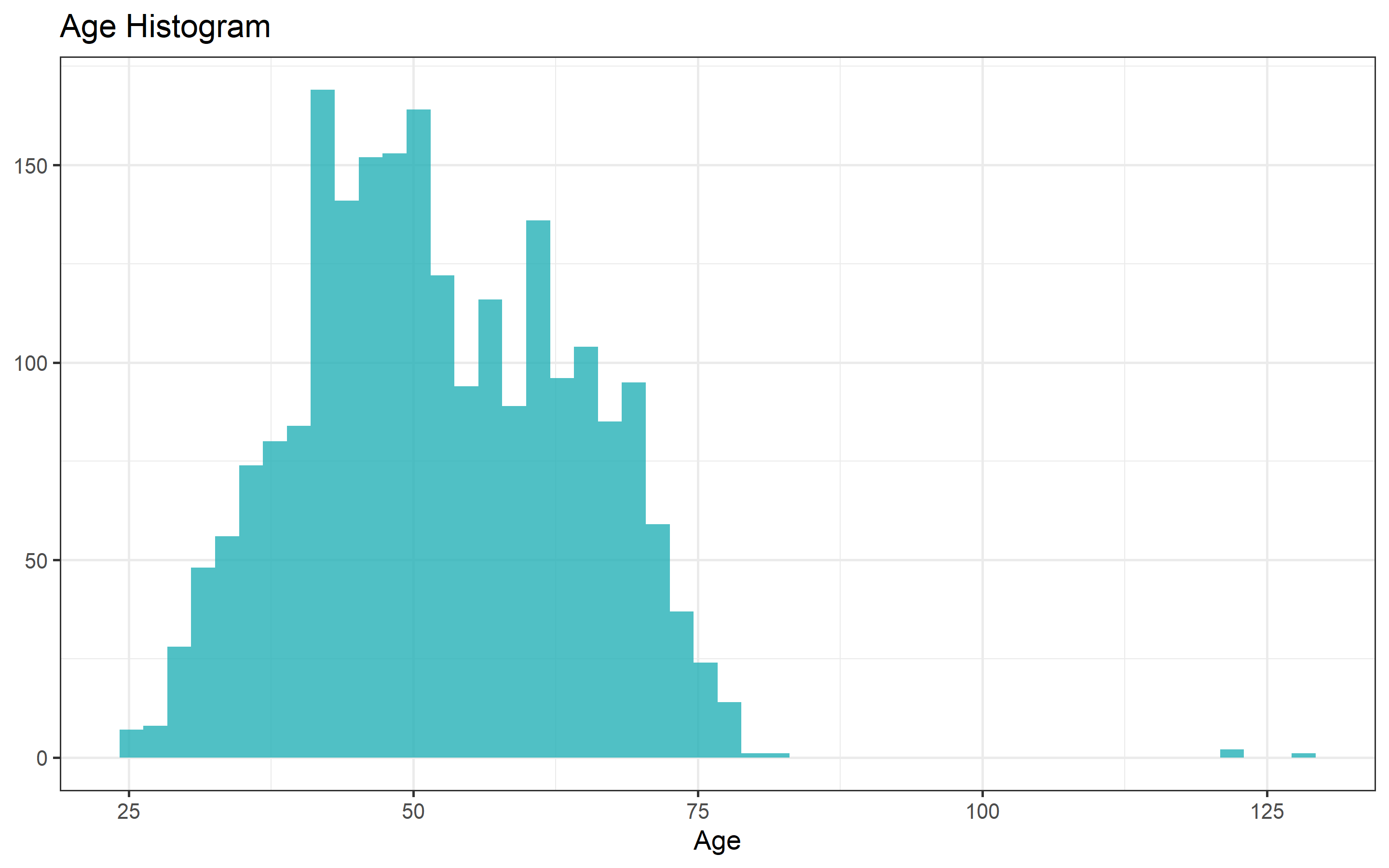
sum(marketing_imp$Age > 100)## [1] 3Three participants older than 100 years old. Since this is a digital commerce, I will drop these observations. It is unlikely that the people in this age buy online.
hist_income <- marketing_imp %>%
  ggplot(aes(Income))+
  geom_histogram(bins = 50, fill = "#24B0B7", alpha = 0.8)+
  labs(title = "Income Histogram")+
  ylab(NULL)
require(scales)
hist_income + scale_x_continuous(labels = comma)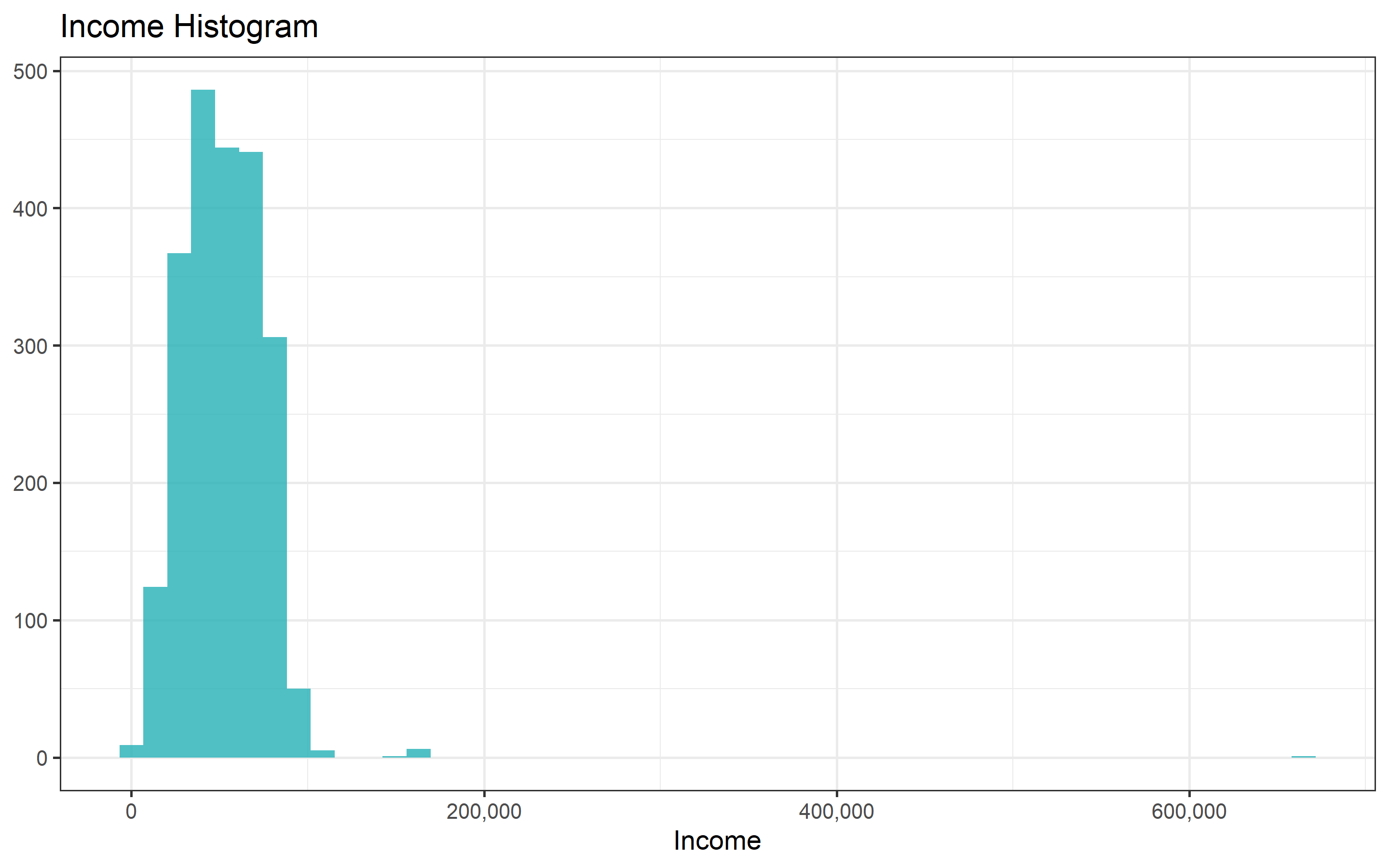
sum(marketing_imp$Income > 100000 )## [1] 13There are 13 participants that earn more than $100,000 dollars per year. I will also drop these observations as they might induce noise to the analyses.
marketing_ready <- marketing_imp %>%
  filter(Income < 100000 & Age < 100)
summary(marketing_ready)
## ID Year_Birth Education Marital_Status
## Min. : 0 Min. :1940 2n Cycle : 201 Married :861
## 1st Qu.: 2828 1st Qu.:1959 Basic : 54 Together:573
## Median : 5458 Median :1970 Graduation:1121 Single :477
## Mean : 5589 Mean :1969 Master : 369 Divorced:229
## 3rd Qu.: 8422 3rd Qu.:1977 PhD : 479 Widow : 77
## Max. :11191 Max. :1996 Alone : 3
## (Other) : 4
## Income Kidhome Teenhome Dt_Customer
## Min. : 1730 Min. :0.0000 Min. :0.0000 Min. :2012-07-30
## 1st Qu.:35376 1st Qu.:0.0000 1st Qu.:0.0000 1st Qu.:2013-01-16
## Median :51412 Median :0.0000 Median :0.0000 Median :2013-07-09
## Mean :51515 Mean :0.4456 Mean :0.5085 Mean :2013-07-10
## 3rd Qu.:67911 3rd Qu.:1.0000 3rd Qu.:1.0000 3rd Qu.:2013-12-30
## Max. :98777 Max. :2.0000 Max. :2.0000 Max. :2014-06-29
##
## Recency MntWines MntFruits MntMeatProducts
## Min. : 0.00 Min. : 0.0 Min. : 0.00 Min. : 0.0
## 1st Qu.:24.00 1st Qu.: 24.0 1st Qu.: 1.75 1st Qu.: 16.0
## Median :49.50 Median : 176.0 Median : 8.00 Median : 67.0
## Mean :49.14 Mean : 304.5 Mean : 26.23 Mean : 165.3
## 3rd Qu.:74.00 3rd Qu.: 504.2 3rd Qu.: 33.00 3rd Qu.: 231.2
## Max. :99.00 Max. :1493.0 Max. :199.00 Max. :1725.0
##
## MntFishProducts MntSweetProducts MntGoldProds NumDealsPurchases
## Min. : 0.00 Min. : 0.00 Min. : 0.00 Min. : 0.000
## 1st Qu.: 3.00 1st Qu.: 1.00 1st Qu.: 9.00 1st Qu.: 1.000
## Median : 12.00 Median : 8.00 Median : 24.00 Median : 2.000
## Mean : 37.57 Mean : 26.91 Mean : 43.95 Mean : 2.325
## 3rd Qu.: 50.00 3rd Qu.: 33.00 3rd Qu.: 56.00 3rd Qu.: 3.000
## Max. :259.00 Max. :263.00 Max. :362.00 Max. :15.000
##
## NumWebPurchases NumCatalogPurchases NumStorePurchases NumWebVisitsMonth
## Min. : 0.000 Min. : 0.000 Min. : 0.000 Min. : 0.000
## 1st Qu.: 2.000 1st Qu.: 0.000 1st Qu.: 3.000 1st Qu.: 3.000
## Median : 4.000 Median : 2.000 Median : 5.000 Median : 6.000
## Mean : 4.085 Mean : 2.627 Mean : 5.804 Mean : 5.341
## 3rd Qu.: 6.000 3rd Qu.: 4.000 3rd Qu.: 8.000 3rd Qu.: 7.000
## Max. :27.000 Max. :28.000 Max. :13.000 Max. :20.000
##
## AcceptedCmp3 AcceptedCmp4 AcceptedCmp5 AcceptedCmp1 AcceptedCmp2 Response
## 0:2061 0:2060 0:2066 0:2084 0:2195 0:1894
## 1: 163 1: 164 1: 158 1: 140 1: 29 1: 330
##
##
##
##
##
## Complain Country Age
## Min. :0.000000 SP :1089 Min. :25.00
## 1st Qu.:0.000000 SA : 332 1st Qu.:44.00
## Median :0.000000 CA : 266 Median :51.00
## Mean :0.008993 AUS : 160 Mean :52.11
## 3rd Qu.:0.000000 IND : 146 3rd Qu.:62.00
## Max. :1.000000 GER : 120 Max. :81.00
## (Other): 111marketing_ready %>%
ggplot(aes(Age))+
geom_histogram(bins = 50, fill = "#24B0B7", alpha = 0.8)+
labs(title = "Age Histogram")+
ylab(NULL)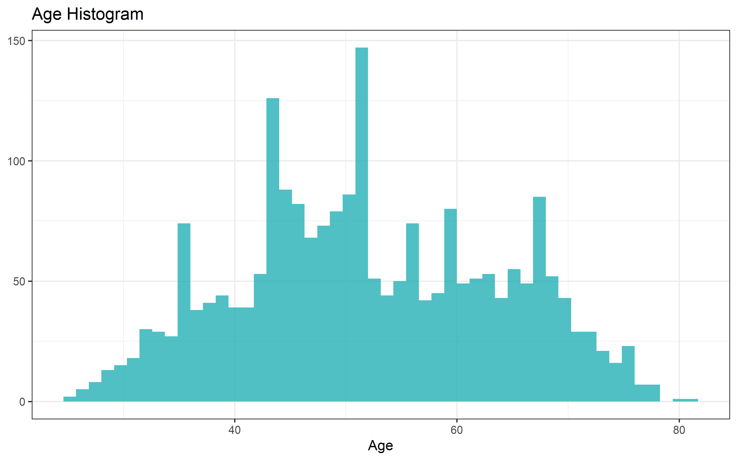
marketing_ready %>%
  ggplot(aes(Income))+
  geom_histogram(bins = 50, fill = "#24B0B7", alpha = 0.8)+
  labs(title = "Income Histogram")+
  ylab(NULL) + scale_x_continuous(labels = comma)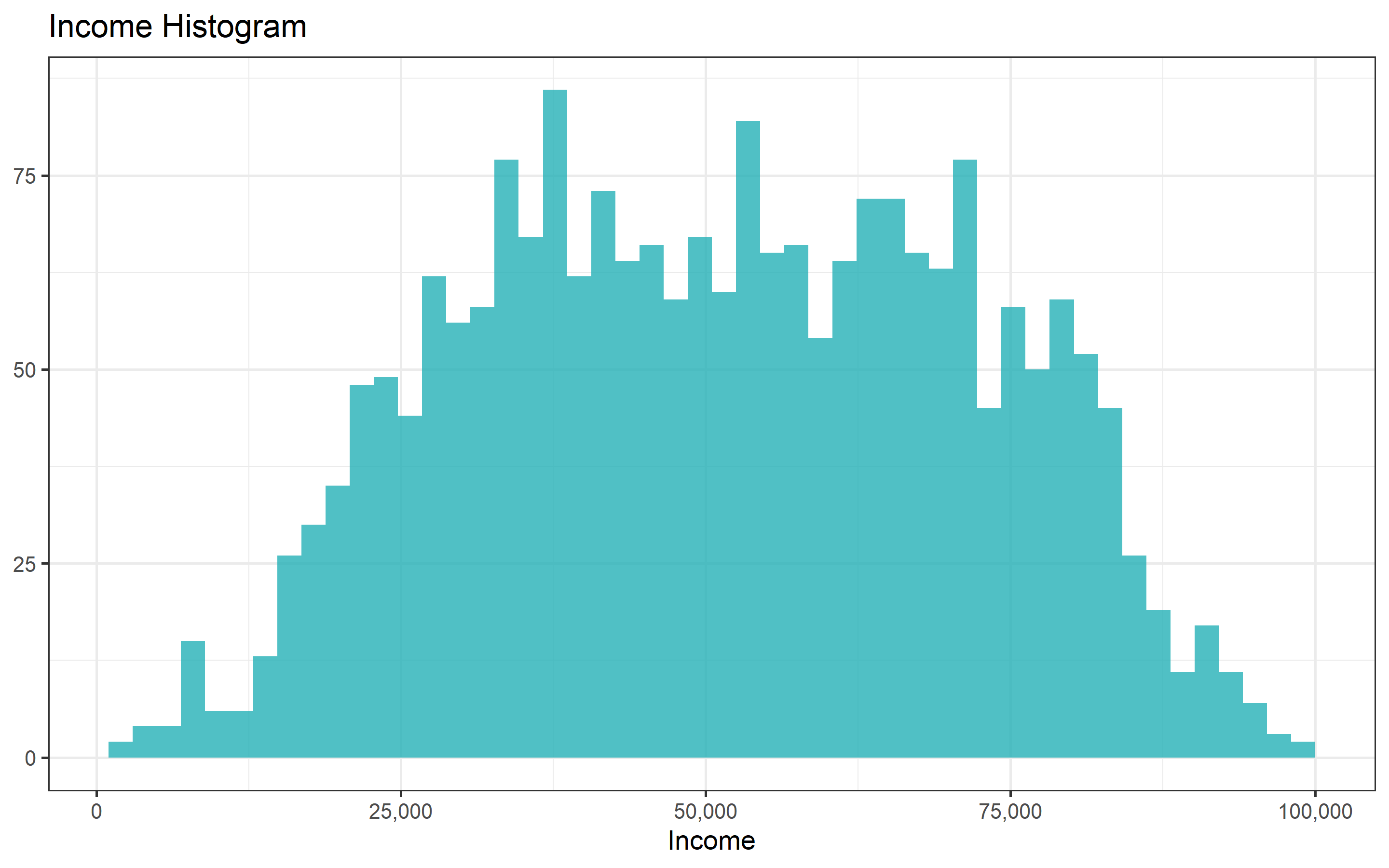
Both variables look better now. Now lets look at the distribution of the remaining continous variables and categorical variables.
hist_wines <- marketing_ready %>%
ggplot(aes(MntWines))+
geom_histogram(bins = 50, fill = "#24B0B7", alpha = 0.8)+
labs(title = "Wine Histogram")+
ylab(NULL) + scale_x_continuous(labels = comma)
hist_fruits <- marketing_ready %>%
ggplot(aes(MntFruits))+
geom_histogram(bins = 50, fill = "#24B0B7", alpha = 0.8)+
labs(title = "Fruits Histogram")+
ylab(NULL) + scale_x_continuous(labels = comma)
hist_MeatProducts <- marketing_ready %>%
ggplot(aes(MntMeatProducts))+
geom_histogram(bins = 50, fill = "#24B0B7", alpha = 0.8)+
labs(title = "Meat Products Histogram")+
ylab(NULL) + scale_x_continuous(labels = comma)
hist_FishProducts <- marketing_ready %>%
ggplot(aes(MntFishProducts))+
geom_histogram(bins = 50, fill = "#24B0B7", alpha = 0.8)+
labs(title = "Fish Products Histogram")+
ylab(NULL) + scale_x_continuous(labels = comma)
hist_SweetProducts <- marketing_ready %>%
ggplot(aes(MntSweetProducts))+
geom_histogram(bins = 50, fill = "#24B0B7", alpha = 0.8)+
labs(title = "Sweet Products Histogram")+
ylab(NULL) + scale_x_continuous(labels = comma)
hist_GoldProds <- marketing_ready %>%
ggplot(aes(MntGoldProds))+
geom_histogram(bins = 50, fill = "#24B0B7", alpha = 0.8)+
labs(title = "Gold Products Histogram")+
ylab(NULL) + scale_x_continuous(labels = comma)
grid.arrange(hist_wines, hist_fruits, hist_MeatProducts, hist_FishProducts,
hist_SweetProducts, hist_GoldProds, ncol=3)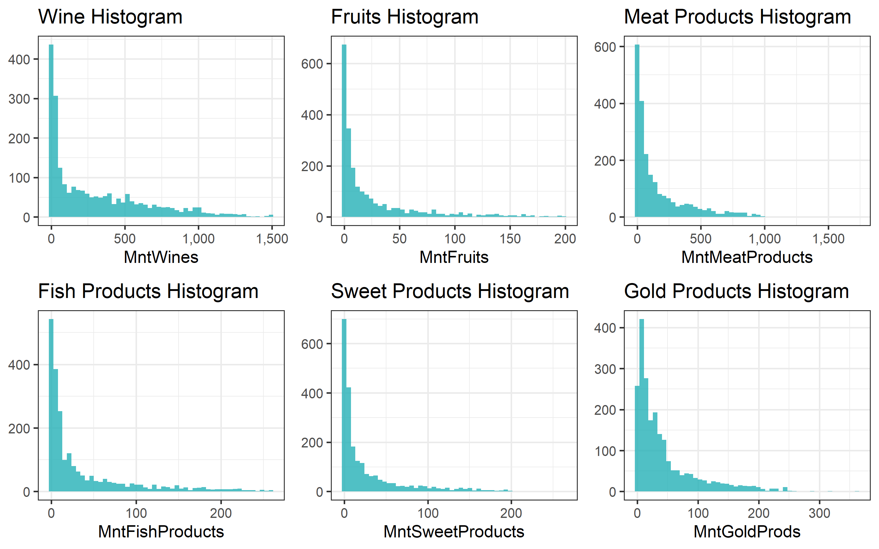 There are a lot of zeros for the distribution of the amount spend on each of the products. A few outliers in the expenditure behavior of the costumers. For example, the meat products histogram shows a point at the right of the distribution with more than 1,500 USD spent in the last two years. The sweet products histogram shows a similar behavior. The gold products are more sold, they have at least higher number of observations with one dollar spent.
par(mfrow = c(3,3))
plot(marketing_ready$Education, main = "Education")
plot(marketing_ready$Marital_Status, main = "Marital Status")
plot(marketing_ready$Country, main = "Country")
plot(marketing_ready$AcceptedCmp1, main = "Offer 1st Campaign Success")
plot(marketing_ready$AcceptedCmp2, main = "Offer 2nd Campaign Success")
plot(marketing_ready$AcceptedCmp3, main = "Offer 3rd Campaign Success")
plot(marketing_ready$AcceptedCmp4, main = "Offer 4th Campaign Success")
plot(marketing_ready$AcceptedCmp1, main = "Offer 5th Campaign Success")
plot(marketing_ready$Response, main = "Last offer Success")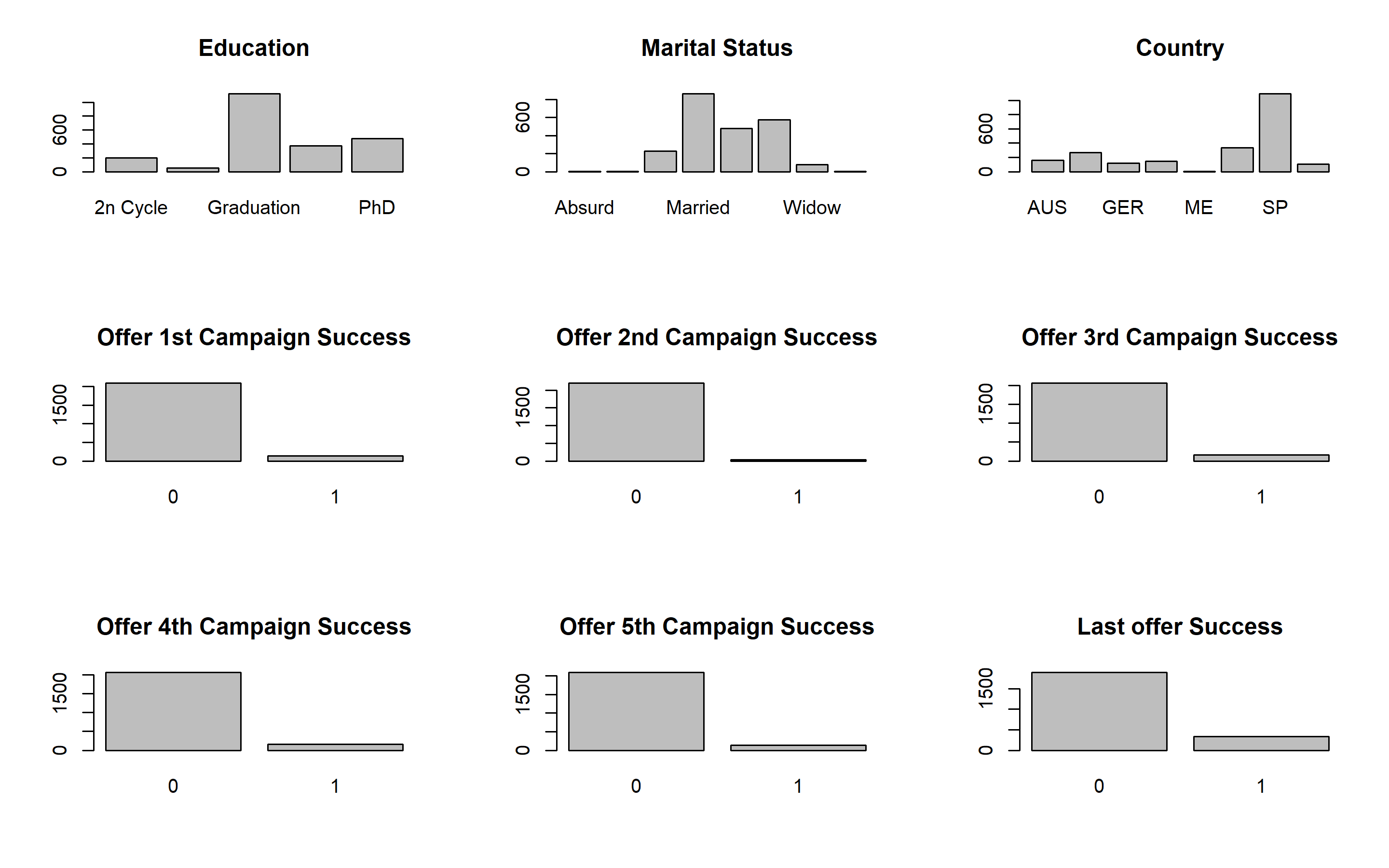
table(marketing_ready$Marital_Status)##
## Absurd Alone Divorced Married Single Together Widow YOLO
## 2 3 229 861 477 573 77 2Probably would make sense to merge Alone with the Single category and drop “Absurd” and “YOLO”.
marketing_ready$Marital_Status <- as.factor(ifelse(as.character(marketing_ready$Marital_Status) == "Alone", "Single",as.character(marketing_ready$Marital_Status)))
table(marketing_ready$Marital_Status)
##
## Absurd Divorced Married Single Together Widow YOLO
## 2 229 861 480 573 77 2marketing_ready <- marketing_ready %>%
filter(Marital_Status != "Absurd" & Marital_Status != "YOLO") %>%
mutate(Marital_Status = factor(Marital_Status))
summary(marketing_ready)## ID Year_Birth Education Marital_Status
## Min. : 0 Min. :1940 2n Cycle : 201 Divorced:229
## 1st Qu.: 2828 1st Qu.:1959 Basic : 54 Married :861
## Median : 5458 Median :1970 Graduation:1120 Single :480
## Mean : 5588 Mean :1969 Master : 368 Together:573
## 3rd Qu.: 8422 3rd Qu.:1977 PhD : 477 Widow : 77
## Max. :11191 Max. :1996
##
## Income Kidhome Teenhome Dt_Customer
## Min. : 1730 Min. :0.0000 Min. :0.0000 Min. :2012-07-30
## 1st Qu.:35336 1st Qu.:0.0000 1st Qu.:0.0000 1st Qu.:2013-01-16
## Median :51412 Median :0.0000 Median :0.0000 Median :2013-07-09
## Mean :51499 Mean :0.4464 Mean :0.5086 Mean :2013-07-10
## 3rd Qu.:67911 3rd Qu.:1.0000 3rd Qu.:1.0000 3rd Qu.:2013-12-30
## Max. :98777 Max. :2.0000 Max. :2.0000 Max. :2014-06-29
##
## Recency MntWines MntFruits MntMeatProducts
## Min. : 0.00 Min. : 0.0 Min. : 0.0 Min. : 0.0
## 1st Qu.:24.00 1st Qu.: 24.0 1st Qu.: 1.0 1st Qu.: 16.0
## Median :50.00 Median : 174.5 Median : 8.0 Median : 67.0
## Mean :49.18 Mean : 304.4 Mean : 26.2 Mean : 165.3
## 3rd Qu.:74.00 3rd Qu.: 505.0 3rd Qu.: 33.0 3rd Qu.: 231.2
## Max. :99.00 Max. :1493.0 Max. :199.0 Max. :1725.0
##
## MntFishProducts MntSweetProducts MntGoldProds NumDealsPurchases
## Min. : 0.00 Min. : 0.00 Min. : 0.00 Min. : 0.000
## 1st Qu.: 3.00 1st Qu.: 1.00 1st Qu.: 9.00 1st Qu.: 1.000
## Median : 12.00 Median : 8.00 Median : 24.00 Median : 2.000
## Mean : 37.45 Mean : 26.92 Mean : 43.81 Mean : 2.323
## 3rd Qu.: 50.00 3rd Qu.: 33.00 3rd Qu.: 56.00 3rd Qu.: 3.000
## Max. :259.00 Max. :263.00 Max. :362.00 Max. :15.000
##
## NumWebPurchases NumCatalogPurchases NumStorePurchases NumWebVisitsMonth
## Min. : 0.000 Min. : 0.000 Min. : 0.000 Min. : 0.000
## 1st Qu.: 2.000 1st Qu.: 0.000 1st Qu.: 3.000 1st Qu.: 3.000
## Median : 4.000 Median : 2.000 Median : 5.000 Median : 6.000
## Mean : 4.082 Mean : 2.624 Mean : 5.803 Mean : 5.342
## 3rd Qu.: 6.000 3rd Qu.: 4.000 3rd Qu.: 8.000 3rd Qu.: 7.000
## Max. :27.000 Max. :28.000 Max. :13.000 Max. :20.000
##
## AcceptedCmp3 AcceptedCmp4 AcceptedCmp5 AcceptedCmp1 AcceptedCmp2 Response
## 0:2057 0:2056 0:2063 0:2081 0:2191 0:1892
## 1: 163 1: 164 1: 157 1: 139 1: 29 1: 328
##
##
##
##
##
## Complain Country Age
## Min. :0.000000 SP :1089 Min. :25.00
## 1st Qu.:0.000000 SA : 332 1st Qu.:44.00
## Median :0.000000 CA : 264 Median :51.00
## Mean :0.009009 AUS : 159 Mean :52.12
## 3rd Qu.:0.000000 IND : 145 3rd Qu.:62.00
## Max. :1.000000 GER : 120 Max. :81.00
## (Other): 111We could also create a variable for total purchases in the last two years
marketing_ready <- marketing_ready %>%
  mutate(total_purch = MntWines + MntFruits + MntMeatProducts + MntFishProducts + MntSweetProducts + MntGoldProds)
marketing_ready %>%
  ggplot(aes(total_purch)) +
  geom_histogram()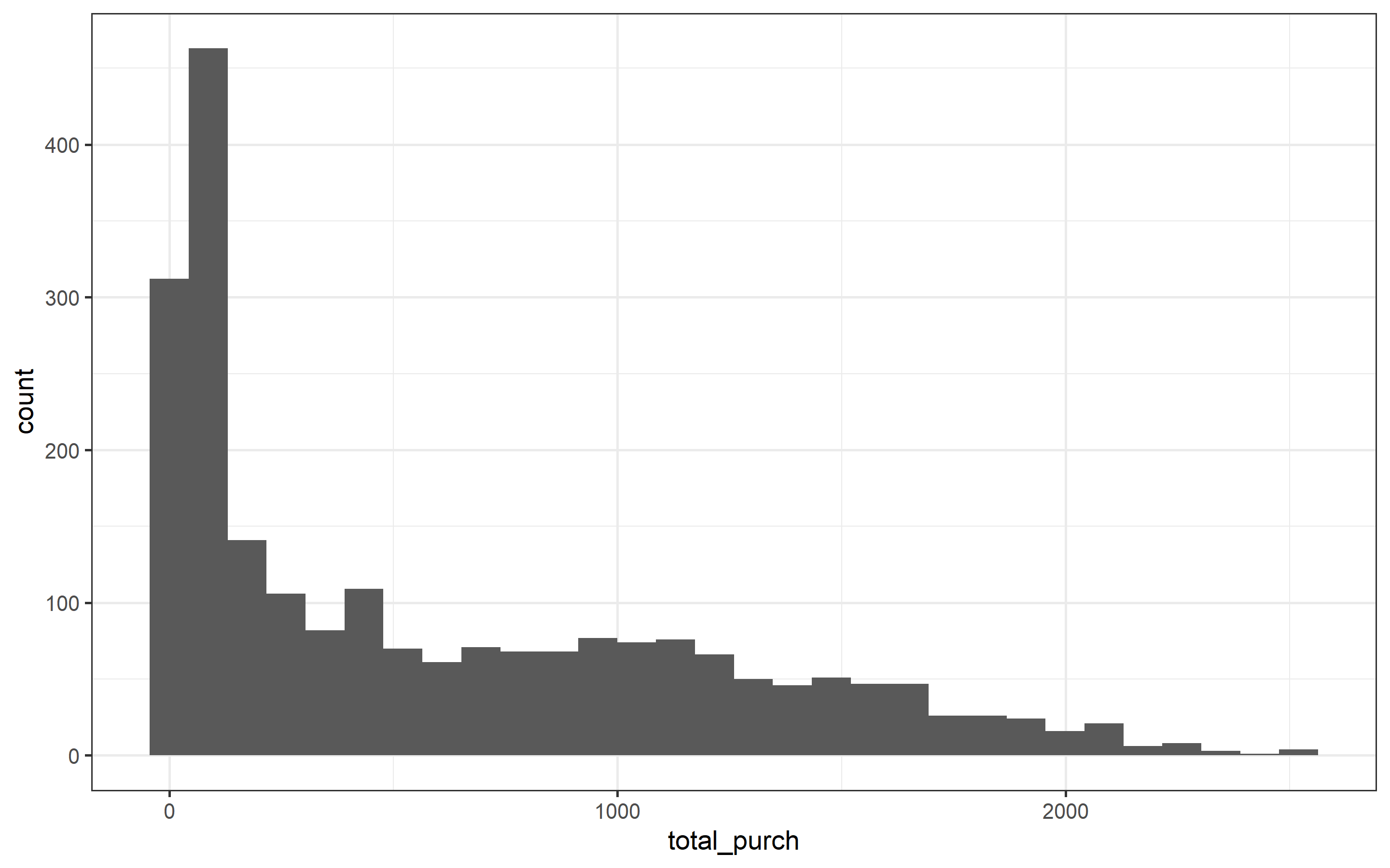
summary(marketing_ready)## ID Year_Birth Education Marital_Status
## Min. : 0 Min. :1940 2n Cycle : 201 Divorced:229
## 1st Qu.: 2828 1st Qu.:1959 Basic : 54 Married :861
## Median : 5458 Median :1970 Graduation:1120 Single :480
## Mean : 5588 Mean :1969 Master : 368 Together:573
## 3rd Qu.: 8422 3rd Qu.:1977 PhD : 477 Widow : 77
## Max. :11191 Max. :1996
##
## Income Kidhome Teenhome Dt_Customer
## Min. : 1730 Min. :0.0000 Min. :0.0000 Min. :2012-07-30
## 1st Qu.:35336 1st Qu.:0.0000 1st Qu.:0.0000 1st Qu.:2013-01-16
## Median :51412 Median :0.0000 Median :0.0000 Median :2013-07-09
## Mean :51499 Mean :0.4464 Mean :0.5086 Mean :2013-07-10
## 3rd Qu.:67911 3rd Qu.:1.0000 3rd Qu.:1.0000 3rd Qu.:2013-12-30
## Max. :98777 Max. :2.0000 Max. :2.0000 Max. :2014-06-29
##
## Recency MntWines MntFruits MntMeatProducts
## Min. : 0.00 Min. : 0.0 Min. : 0.0 Min. : 0.0
## 1st Qu.:24.00 1st Qu.: 24.0 1st Qu.: 1.0 1st Qu.: 16.0
## Median :50.00 Median : 174.5 Median : 8.0 Median : 67.0
## Mean :49.18 Mean : 304.4 Mean : 26.2 Mean : 165.3
## 3rd Qu.:74.00 3rd Qu.: 505.0 3rd Qu.: 33.0 3rd Qu.: 231.2
## Max. :99.00 Max. :1493.0 Max. :199.0 Max. :1725.0
##
## MntFishProducts MntSweetProducts MntGoldProds NumDealsPurchases
## Min. : 0.00 Min. : 0.00 Min. : 0.00 Min. : 0.000
## 1st Qu.: 3.00 1st Qu.: 1.00 1st Qu.: 9.00 1st Qu.: 1.000
## Median : 12.00 Median : 8.00 Median : 24.00 Median : 2.000
## Mean : 37.45 Mean : 26.92 Mean : 43.81 Mean : 2.323
## 3rd Qu.: 50.00 3rd Qu.: 33.00 3rd Qu.: 56.00 3rd Qu.: 3.000
## Max. :259.00 Max. :263.00 Max. :362.00 Max. :15.000
##
## NumWebPurchases NumCatalogPurchases NumStorePurchases NumWebVisitsMonth
## Min. : 0.000 Min. : 0.000 Min. : 0.000 Min. : 0.000
## 1st Qu.: 2.000 1st Qu.: 0.000 1st Qu.: 3.000 1st Qu.: 3.000
## Median : 4.000 Median : 2.000 Median : 5.000 Median : 6.000
## Mean : 4.082 Mean : 2.624 Mean : 5.803 Mean : 5.342
## 3rd Qu.: 6.000 3rd Qu.: 4.000 3rd Qu.: 8.000 3rd Qu.: 7.000
## Max. :27.000 Max. :28.000 Max. :13.000 Max. :20.000
##
## AcceptedCmp3 AcceptedCmp4 AcceptedCmp5 AcceptedCmp1 AcceptedCmp2 Response
## 0:2057 0:2056 0:2063 0:2081 0:2191 0:1892
## 1: 163 1: 164 1: 157 1: 139 1: 29 1: 328
##
##
##
##
##
## Complain Country Age total_purch
## Min. :0.000000 SP :1089 Min. :25.00 Min. : 5.0
## 1st Qu.:0.000000 SA : 332 1st Qu.:44.00 1st Qu.: 69.0
## Median :0.000000 CA : 264 Median :51.00 Median : 395.5
## Mean :0.009009 AUS : 159 Mean :52.12 Mean : 604.1
## 3rd Qu.:0.000000 IND : 145 3rd Qu.:62.00 3rd Qu.:1039.2
## Max. :1.000000 GER : 120 Max. :81.00 Max. :2525.0
## (Other): 111marketing_ready %>%
ggplot(aes(Income, log(total_purch)))+
geom_point()+
geom_smooth()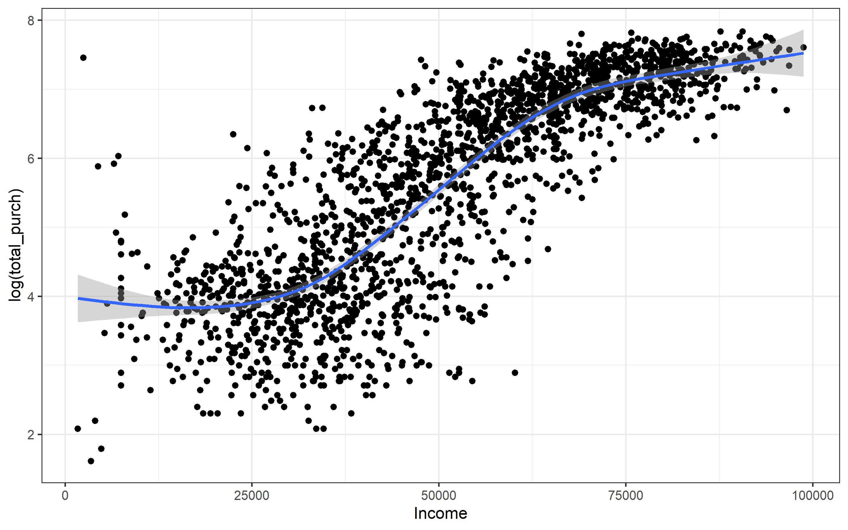 There is a non-linear relationship between amount spent and income.
Section 02: Statistical Analysis
- What factors are significantly related to the number of store purchases?
- Does US fare significantly better than the Rest of the World in terms of total purchases?
- Your supervisor insists that people who buy gold are more conservative. Therefore, people who spent an above average amount on gold in the last 2 years would have more in store purchases. Justify or refute this statement using an appropriate statistical test
- Fish has Omega 3 fatty acids which are good for the brain. Accordingly, do “Married PhD candidates” have a significant relation with amount spent on fish? What other factors are significantly related to amount spent on fish? (Hint: use your knowledge of interaction variables/effects)
- Is there a significant relationship between geographical regional and success of a campaign?
To answer question 1 we can regress the number of store purchases on age, education, marital status, income, number of kids and teenagers at home and country. Also a second regression could include the offers the costumer took. A third regression could also include an indicator variable for each type of product to identify which products are acquired in a store. It is interesting to investigate a count model that estimates the probabilities of the costumers purchasing in a store.
marketing_ready <- marketing_ready %>%
  mutate(wine = factor(ifelse(MntWines > 0, 1, 0)),
         fruits = factor(ifelse(MntFruits > 0, 1, 0)),
         meat = factor(ifelse(MntMeatProducts > 0, 1, 0)),
         fish = factor(ifelse(MntFishProducts > 0, 1, 0)),
         sweet = factor(ifelse(MntSweetProducts > 0, 1, 0)),
         gold = factor(ifelse(MntGoldProds > 0, 1, 0)),
         store_purchase = factor(ifelse(NumStorePurchases > 0, 1,0)))

store_ols1 <- lm(NumStorePurchases ~ Age + Education + Marital_Status + Income + Kidhome + Teenhome + Country, data = marketing_ready)
store_ols2 <- lm(NumStorePurchases ~ Age + Education + Marital_Status + Income + Kidhome + Teenhome + Country + AcceptedCmp1 + AcceptedCmp2 + AcceptedCmp3 + AcceptedCmp4 + AcceptedCmp5 + Response, data = marketing_ready)
store_ols3 <- lm(NumStorePurchases ~ Age + Education + Marital_Status + Income + Kidhome + Teenhome + Country + AcceptedCmp1 + AcceptedCmp2 + AcceptedCmp3 + AcceptedCmp4 + AcceptedCmp5 + Response + wine + fruits + meat + fish + sweet + gold, data = marketing_ready)
store_negbin1 <- glm(NumStorePurchases ~ Age + Education + Marital_Status + Income + Kidhome + Teenhome + Country + AcceptedCmp1 + AcceptedCmp2 + AcceptedCmp3 + AcceptedCmp4 + AcceptedCmp5 + Response + wine + fruits + meat + fish + sweet + gold, family = negative.binomial(theta = 1), data = marketing_ready)
stargazer(store_ols1, store_ols2, store_ols3, store_negbin1, type = "text", align = TRUE, no.space = TRUE)
##
## ===============================================================================================================================
## Dependent variable:
## --------------------------------------------------------------------------------------------------------
## NumStorePurchases
## OLS glm: Negative Binomial(1)
## link = log
## (1) (2) (3) (4)
## -------------------------------------------------------------------------------------------------------------------------------
## Age -0.011** -0.012** -0.010** -0.001*
## (0.005) (0.005) (0.005) (0.001)
## EducationBasic 0.048 0.100 0.062 -0.032
## (0.361) (0.357) (0.358) (0.061)
## EducationGraduation -0.127 -0.122 -0.065 -0.016
## (0.177) (0.175) (0.174) (0.029)
## EducationMaster -0.075 -0.062 0.103 0.022
## (0.204) (0.202) (0.202) (0.033)
## EducationPhD -0.168 -0.132 0.161 0.033
## (0.197) (0.195) (0.200) (0.033)
## Marital_StatusMarried 0.165 0.136 0.163 0.047*
## (0.172) (0.171) (0.169) (0.028)
## Marital_StatusSingle -0.009 -0.013 0.025 0.011
## (0.187) (0.184) (0.183) (0.030)
## Marital_StatusTogether 0.043 -0.014 0.015 0.016
## (0.180) (0.178) (0.177) (0.029)
## Marital_StatusWidow 0.065 0.090 0.132 0.063
## (0.305) (0.301) (0.299) (0.048)
## Income 0.0001*** 0.0001*** 0.0001*** 0.00002***
## (0.00000) (0.00000) (0.00000) (0.00000)
## Kidhome -1.226*** -1.196*** -1.089*** -0.205***
## (0.109) (0.107) (0.108) (0.018)
## Teenhome 0.182* 0.001 0.110 0.048***
## (0.097) (0.099) (0.100) (0.016)
## CountryCA 0.162 0.152 0.114 0.016
## (0.231) (0.228) (0.226) (0.037)
## CountryGER 0.240 0.211 0.228 0.031
## (0.279) (0.275) (0.273) (0.044)
## CountryIND 0.152 0.106 0.151 0.021
## (0.265) (0.262) (0.259) (0.043)
## CountryME -0.338 -0.015 -0.081 0.081
## (1.340) (1.326) (1.315) (0.210)
## CountrySA 0.327 0.302 0.288 0.049
## (0.222) (0.219) (0.217) (0.036)
## CountrySP 0.261 0.278 0.273 0.037
## (0.195) (0.193) (0.192) (0.031)
## CountryUS 0.426 0.401 0.346 0.054
## (0.287) (0.283) (0.281) (0.046)
## AcceptedCmp11 -0.493** -0.446** -0.071**
## (0.227) (0.226) (0.036)
## AcceptedCmp21 0.652 0.871* 0.182**
## (0.451) (0.448) (0.071)
## AcceptedCmp31 -0.472** -0.416** -0.114***
## (0.194) (0.193) (0.032)
## AcceptedCmp41 0.384* 0.573*** 0.116***
## (0.205) (0.205) (0.033)
## AcceptedCmp51 -0.886*** -0.877*** -0.178***
## (0.230) (0.228) (0.036)
## Response1 -0.527*** -0.612*** -0.076***
## (0.154) (0.153) (0.025)
## wine1 0.326 0.116
## (0.673) (0.118)
## fruits1 0.180 0.043*
## (0.144) (0.024)
## meat1 0.248 0.203
## (2.348) (0.426)
## fish1 0.336** 0.075***
## (0.147) (0.024)
## sweet1 0.650*** 0.129***
## (0.142) (0.023)
## gold1 0.425 0.090*
## (0.297) (0.049)
## Constant 1.836*** 1.776*** -0.339 0.215
## (0.404) (0.402) (2.285) (0.415)
## -------------------------------------------------------------------------------------------------------------------------------
## Observations 2,220 2,220 2,220 2,220
## R2 0.502 0.516 0.527
## Adjusted R2 0.497 0.510 0.520
## Log Likelihood -6,128.878
## Akaike Inf. Crit. 12,321.760
## Residual Std. Error 2.293 (df = 2200) 2.263 (df = 2194) 2.241 (df = 2188)
## F Statistic 116.601*** (df = 19; 2200) 93.464*** (df = 25; 2194) 78.542*** (df = 31; 2188)
## ===============================================================================================================================
## Note: *p<0.1; **p<0.05; ***p<0.01The OLS models hint us that the factors driven store purchases are kids and teenagers at home, income, the offer accepted at the moment of the purchase and the product that the costumer buys. The count model confirms these findings. It seems that the second and fourth offer affects positively purchasing in stores. Fish and sweets are the products that also contributes to more purchases. Income follows the same pattern, and surprisingly age contributes negatively to store purchases.
To answer question 2, lets plot a graph to observe how the country contribution to total purchases.
marketing_ready %>%
ggplot(aes(Country, total_purch, fill = Country)) +
geom_col() +
scale_y_continuous() +
coord_flip() +
scale_fill_brewer(palette = "Spectral")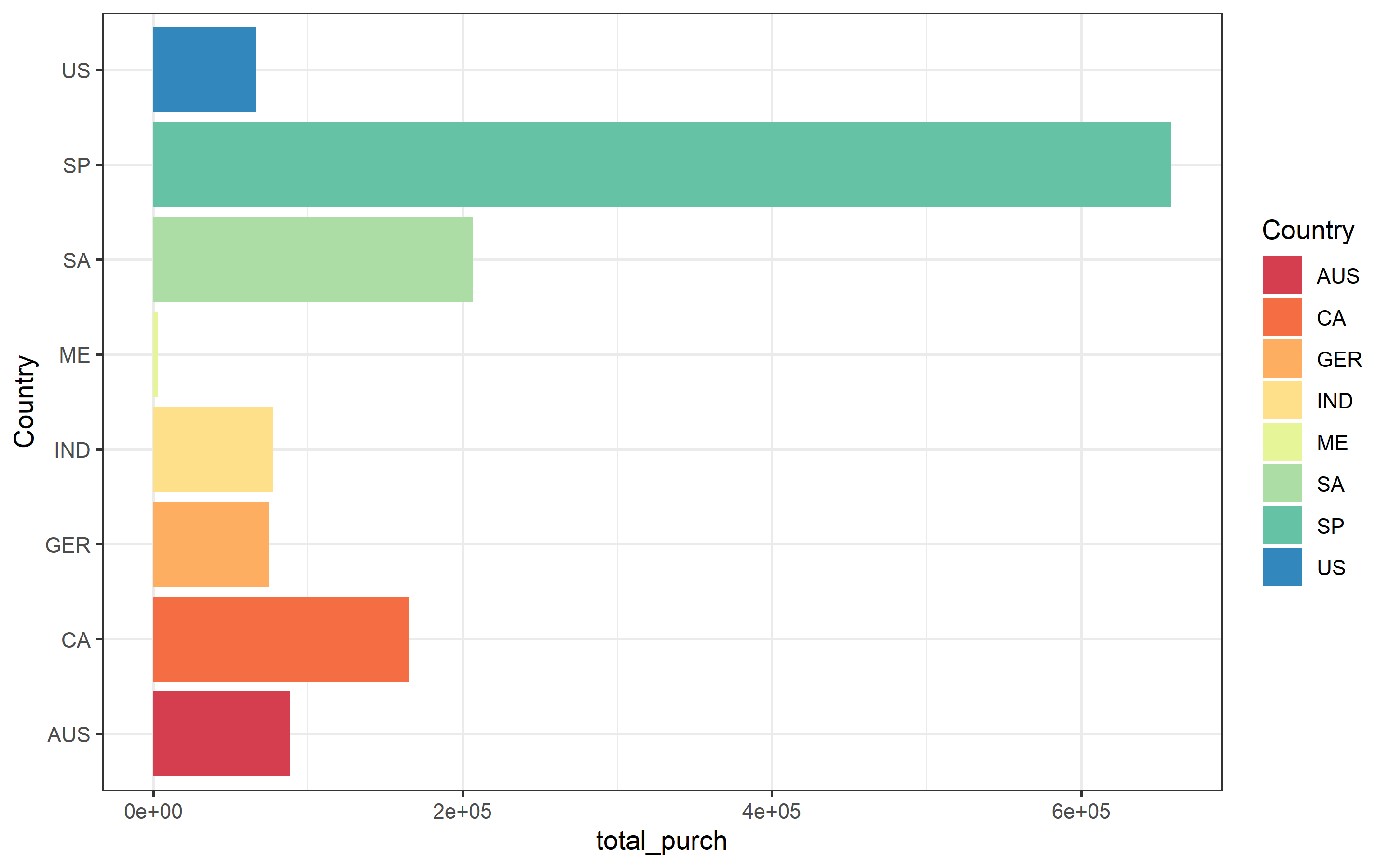 By comparing only countries total purchases, Spain is doing better than any other country. However, Spain is also the country with more costumers.
summary(marketing_ready$Country)## AUS CA GER IND ME SA SP US
## 159 264 120 145 3 332 1089 108Lets use a boxplot to investigate this,
marketing_ready %>%
ggplot(aes(total_purch, Country, fill = Country)) +
geom_boxplot(outlier.alpha = 0.5) +
scale_x_continuous() +
scale_fill_brewer(palette = "Spectral")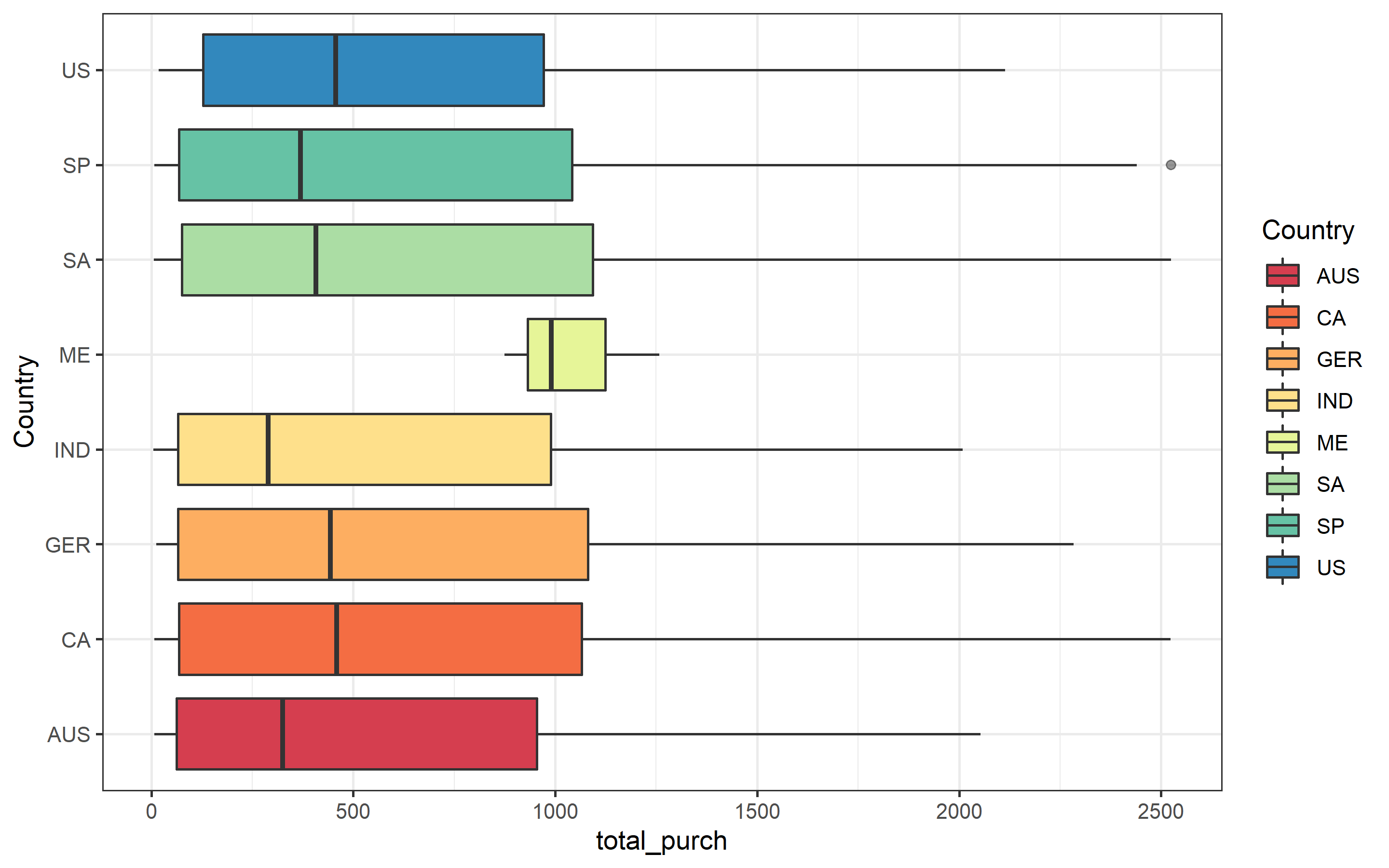 Now we can see that the median of the US is higher than Spain. Mexico is by far the country with more total purchases.
marketing_ready %>%
group_by(Country) %>%
mutate(mean_country = mean(total_purch)) %>%
ggplot(aes(Country, mean_country, colour = Country)) +
geom_point() +
scale_colour_brewer(palette = "Spectral")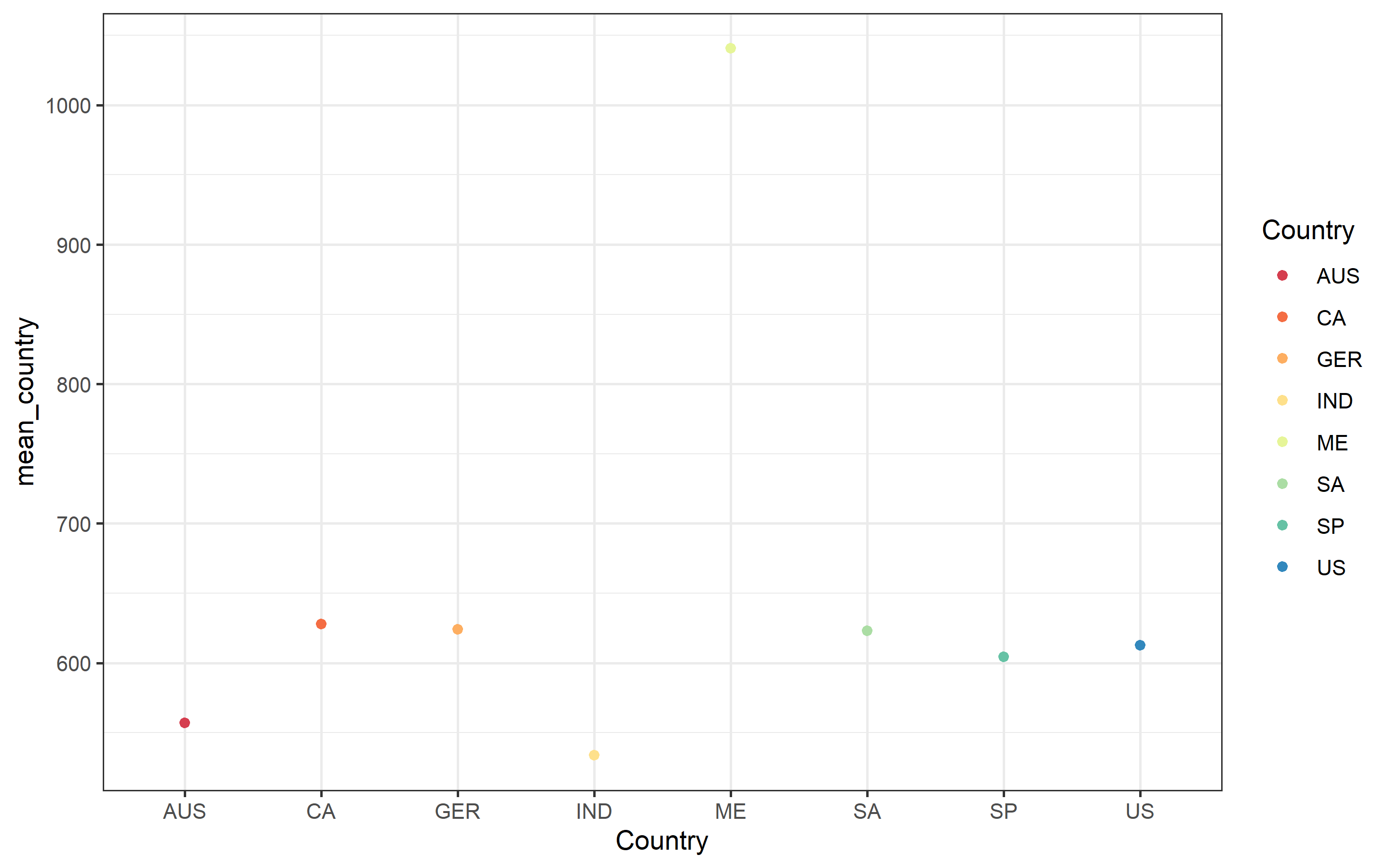 In average, the US has a higher total purchases value than SP, IND and AUS but GER and CA are slightly better than US, and ME is better. We can run a regression to see these effects.
marketing_country <- marketing_ready %>%
  mutate(Country = relevel(Country, ref = "US"))

totalpurch1 <- lm(log(total_purch) ~ Age + Income + I(Income^2) + Country + Kidhome + Teenhome + AcceptedCmp1 + AcceptedCmp1 + AcceptedCmp2 + AcceptedCmp3 + AcceptedCmp4 + AcceptedCmp5 + Response + Complain, data = marketing_country)
stargazer(totalpurch1, type = "text", aling = TRUE, no.space = TRUE)
##
## ===============================================
## Dependent variable:
## ---------------------------
## log(total_purch)
## -----------------------------------------------
## Age -0.003*
## (0.002)
## Income 0.0001***
## (0.00000)
## I(Income2) -0.000***
## (0.000)
## CountryAUS -0.218**
## (0.094)
## CountryCA -0.141
## (0.086)
## CountryGER -0.278***
## (0.100)
## CountryIND -0.096
## (0.096)
## CountryME 0.330
## (0.441)
## CountrySA -0.117
## (0.083)
## CountrySP -0.169**
## (0.076)
## Kidhome -0.661***
## (0.036)
## Teenhome -0.138***
## (0.034)
## AcceptedCmp11 -0.051
## (0.076)
## AcceptedCmp21 -0.067
## (0.149)
## AcceptedCmp31 0.160**
## (0.064)
## AcceptedCmp41 0.277***
## (0.068)
## AcceptedCmp51 -0.232***
## (0.079)
## Response1 0.307***
## (0.050)
## Complain -0.127
## (0.169)
## Constant 3.252***
## (0.142)
## -----------------------------------------------
## Observations 2,220
## R2 0.744
## Adjusted R2 0.742
## Residual Std. Error 0.751 (df = 2200)
## F Statistic 337.264*** (df = 19; 2200)
## ===============================================
## Note: *p<0.1; **p<0.05; ***p<0.01
##
## ====
## TRUE
## ----What we have found with the regression analysis is that average total purchases in AUS, GER and SP are lower than in the US. In average, AUS total purchases are 21.8% lower compared to the US. Same pattern for GER and SP, 27.8% and 16.9% lower.
To answer question, we create an indicator variable that equals 1 whether the amount spent on gold is higher than the average or not. Then regress the number of store purchases on this indicator variable. The mean of the amount spend on gold is 43.81.
summary(marketing_ready$MntGoldProds)## Min. 1st Qu. Median Mean 3rd Qu. Max.
## 0.00 9.00 24.00 43.81 56.00 362.00marketing_ready <- marketing_ready %>%
mutate(gold_above = as.factor(ifelse(MntGoldProds > 45, 1, 0)))
summary(marketing_ready$gold_above)## 0 1
## 1549 671above1 <- lm(NumStorePurchases ~ Age + Education + Marital_Status + Income + Kidhome + Teenhome + Country + AcceptedCmp1 + AcceptedCmp2 + AcceptedCmp3 + AcceptedCmp4 + AcceptedCmp5 + Response + gold_above, data = marketing_ready)
stargazer(above1, type = "text", no.space = TRUE, align = TRUE)##
## ==================================================
## Dependent variable:
## ---------------------------
## NumStorePurchases
## --------------------------------------------------
## Age -0.011**
## (0.005)
## EducationBasic 0.071
## (0.352)
## EducationGraduation -0.138
## (0.173)
## EducationMaster -0.034
## (0.199)
## EducationPhD 0.026
## (0.194)
## Marital_StatusMarried 0.137
## (0.169)
## Marital_StatusSingle 0.017
## (0.182)
## Marital_StatusTogether -0.008
## (0.176)
## Marital_StatusWidow -0.011
## (0.298)
## Income 0.0001***
## (0.00000)
## Kidhome -1.081***
## (0.107)
## Teenhome 0.002
## (0.098)
## CountryCA 0.165
## (0.225)
## CountryGER 0.187
## (0.272)
## CountryIND 0.077
## (0.259)
## CountryME 0.097
## (1.310)
## CountrySA 0.307
## (0.216)
## CountrySP 0.289
## (0.191)
## CountryUS 0.438
## (0.280)
## AcceptedCmp11 -0.447**
## (0.225)
## AcceptedCmp21 0.546
## (0.446)
## AcceptedCmp31 -0.582***
## (0.192)
## AcceptedCmp41 0.506**
## (0.203)
## AcceptedCmp51 -0.814***
## (0.227)
## Response1 -0.583***
## (0.153)
## gold_above1 0.878***
## (0.118)
## Constant 1.753***
## (0.397)
## --------------------------------------------------
## Observations 2,220
## R2 0.528
## Adjusted R2 0.522
## Residual Std. Error 2.236 (df = 2193)
## F Statistic 94.207*** (df = 26; 2193)
## ==================================================
## Note: *p<0.1; **p<0.05; ***p<0.01The result of the regression confirms the supervisor’s hypothesis. Among gold buyers, those who buy more than the average go more often to the store.
Lets now analyze question 4. To investigate that, I will run a regression interacting marital status and education. To answer it correctly, the reference category for marital status is “married” and for education “PhD”. In this sense, we can compare the categories with the other ones.
marketing_ready <- marketing_ready %>%
  mutate(Marital_Status = relevel(Marital_Status, ref = "Married"),
         Education = relevel(Education, ref = "PhD"))
inter1 <- lm(MntFishProducts ~ 0 + Age + Education + Marital_Status + Education*Marital_Status + Income + I(Income^2) + Kidhome + Teenhome + Country + AcceptedCmp1 + AcceptedCmp2 + AcceptedCmp3 + AcceptedCmp4 + AcceptedCmp5 + Response, data = marketing_ready)
stargazer(inter1, type = "text", no.space = TRUE, align = TRUE)
##
## ======================================================================
## Dependent variable:
## ---------------------------
## MntFishProducts
## ----------------------------------------------------------------------
## Age 0.039
## (0.086)
## EducationPhD -6.957
## (8.620)
## Education2n Cycle 13.651
## (8.828)
## EducationBasic 25.293**
## (11.293)
## EducationGraduation 11.571
## (7.983)
## EducationMaster -4.701
## (8.700)
## Marital_StatusDivorced 12.934**
## (6.465)
## Marital_StatusSingle -1.338
## (5.135)
## Marital_StatusTogether -3.500
## (4.877)
## Marital_StatusWidow 3.553
## (8.950)
## Income -0.00002
## (0.0002)
## I(Income2) 0.00000***
## (0.000)
## Kidhome -12.360***
## (1.956)
## Teenhome -18.226***
## (1.881)
## CountryCA -0.148
## (4.149)
## CountryGER -0.980
## (5.000)
## CountryIND 0.713
## (4.754)
## CountryME 32.870
## (24.019)
## CountrySA 3.831
## (3.979)
## CountrySP 0.773
## (3.512)
## CountryUS 1.292
## (5.138)
## AcceptedCmp11 15.009***
## (4.168)
## AcceptedCmp21 -11.646
## (8.192)
## AcceptedCmp31 -0.569
## (3.536)
## AcceptedCmp41 -19.617***
## (3.710)
## AcceptedCmp51 -28.824***
## (4.359)
## Response1 1.474
## (2.808)
## Education2n Cycle:Marital_StatusDivorced -18.771
## (11.813)
## EducationBasic:Marital_StatusDivorced -18.634
## (42.554)
## EducationGraduation:Marital_StatusDivorced -20.065***
## (7.727)
## EducationMaster:Marital_StatusDivorced -8.141
## (9.966)
## Education2n Cycle:Marital_StatusSingle -8.880
## (9.695)
## EducationBasic:Marital_StatusSingle -8.365
## (14.306)
## EducationGraduation:Marital_StatusSingle 1.416
## (6.064)
## EducationMaster:Marital_StatusSingle 9.494
## (7.798)
## Education2n Cycle:Marital_StatusTogether 28.614***
## (8.613)
## EducationBasic:Marital_StatusTogether -13.129
## (15.114)
## EducationGraduation:Marital_StatusTogether 5.623
## (5.803)
## EducationMaster:Marital_StatusTogether 10.993
## (7.219)
## Education2n Cycle:Marital_StatusWidow 51.207**
## (20.899)
## EducationBasic:Marital_StatusWidow -4.079
## (43.011)
## EducationGraduation:Marital_StatusWidow -1.078
## (11.450)
## EducationMaster:Marital_StatusWidow 39.894***
## (15.243)
## ----------------------------------------------------------------------
## Observations 2,220
## R2 0.624
## Adjusted R2 0.616
## Residual Std. Error 40.930 (df = 2177)
## F Statistic 83.899*** (df = 43; 2177)
## ======================================================================
## Note: *p<0.1; **p<0.05; ***p<0.01The results of the regression tell us that married PhD candidates only buy more fish than graduated divorced participants. Widow participants tend to spend more in fish products. In general, divorced participants buy more fish too. Kids and teens at home decrease the amount spent in fish. Those who accepted offer campaign 2 buy more fish. Accepting campaigns 4 and5 spend less in fish than those who did not accept these campaigns.
To answer question 5, we can explore graphically the different campaigns.
par(mfrow = c(2,3))
plot(marketing_ready$AcceptedCmp1 ~ marketing_ready$Country, main = "Campaing 1", ylab = "Accepted Offer", xlab = "Country")
plot(marketing_ready$AcceptedCmp2 ~ marketing_ready$Country, main = "Campaing 2", ylab = NULL, xlab = "Country")
title(ylab = NULL)
plot(marketing_ready$AcceptedCmp3 ~ marketing_ready$Country, main = "Campaing 3", ylab = NULL, xlab = "Country")
plot(marketing_ready$AcceptedCmp4 ~ marketing_ready$Country, main = "Campaing 4", ylab = "Accepted Offer", xlab = "Country")
plot(marketing_ready$AcceptedCmp5 ~ marketing_ready$Country, main = "Campaing 5", ylab = NULL, xlab = "Country")
plot(marketing_ready$Response ~ marketing_ready$Country, main = "Last Campaign", ylab = NULL, xlab = "Country")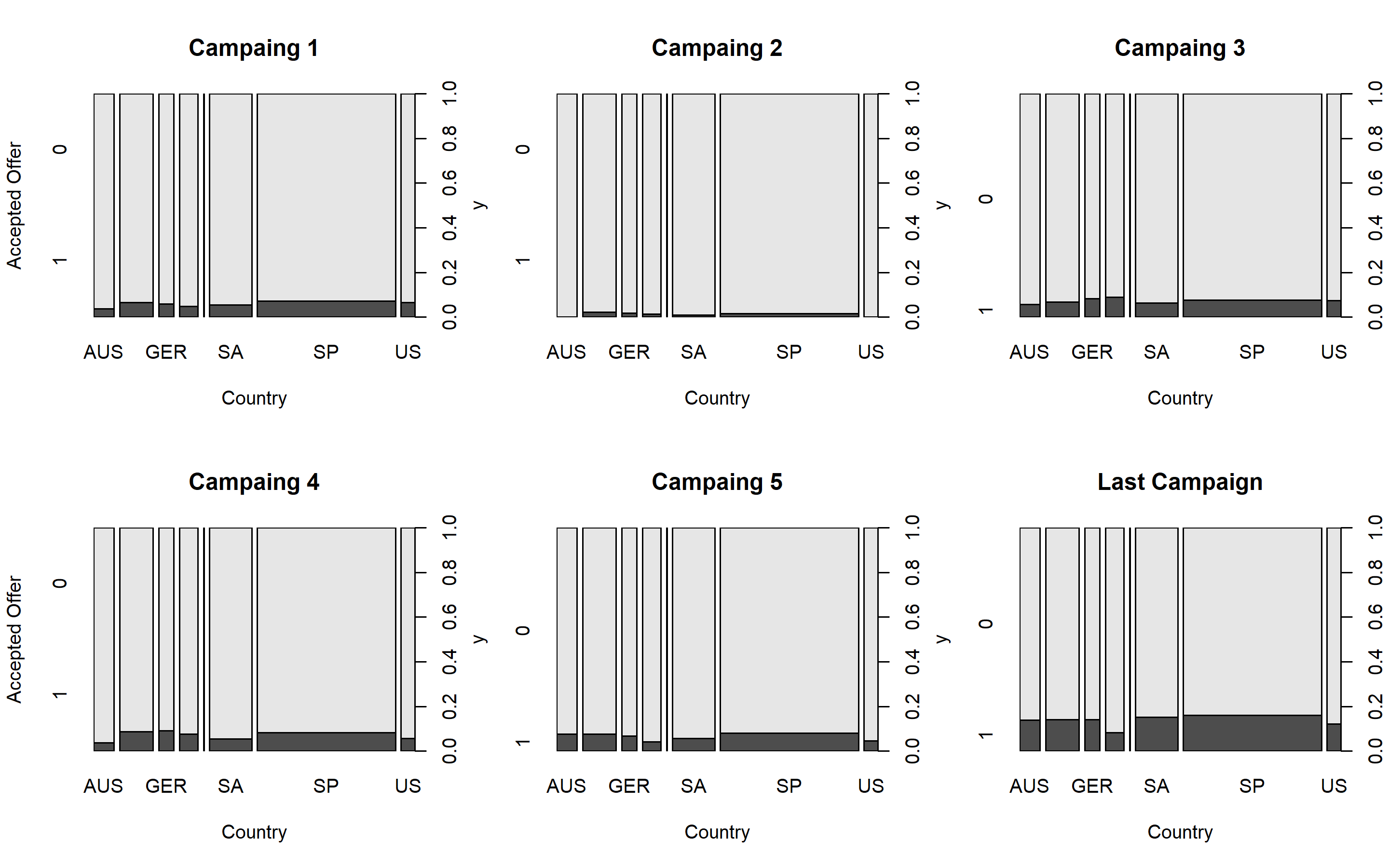
marketing_ready$offers <- ifelse(marketing_ready$AcceptedCmp1 == 1, "1st", 0)
marketing_ready$offers <- ifelse(marketing_ready$AcceptedCmp2 == 1, "2nd", marketing_ready$offers)
marketing_ready$offers <- ifelse(marketing_ready$AcceptedCmp3 == 1, "3rd", marketing_ready$offers)
marketing_ready$offers <- ifelse(marketing_ready$AcceptedCmp4 == 1, "4th", marketing_ready$offers)
marketing_ready$offers <- ifelse(marketing_ready$AcceptedCmp5 == 1, "5th", marketing_ready$offers)
marketing_ready$offers <- ifelse(marketing_ready$Response == 1, "Last", marketing_ready$offers)
marketing_ready$offers <- ifelse(marketing_ready$AcceptedCmp2 == 1, "2nd", marketing_ready$offers)
marketing_ready %>%
filter(offers != 0) %>%
ggplot(aes(offers)) +
geom_bar(fill = c("#24B0B7", "#39D97B", "#825DE3", "#DC8BE7", "#F31E1E", "#231985"), alpha = 0.8) 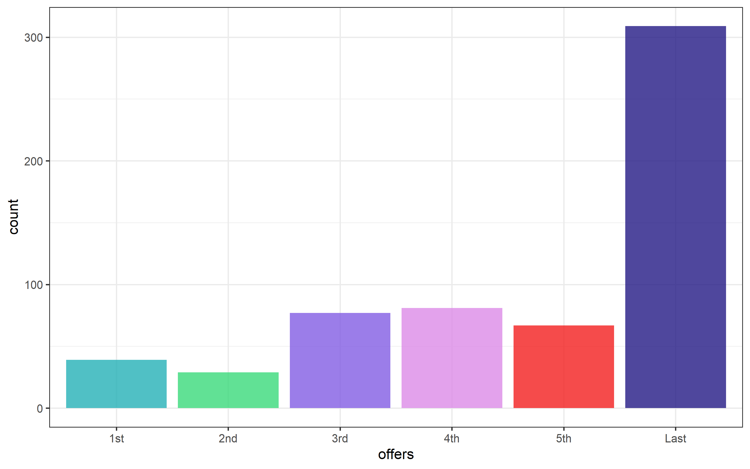 From the campaigns, the last one is the most successful one. Almost three times what others campaigns did. The company could apply another similar campaign to even increase the acceptance rate.
amountspent <- marketing %>%
    dplyr::select(MntWines, MntFruits, MntMeatProducts, MntFishProducts, MntSweetProducts, MntGoldProds) %>%
    mutate(Wines = sum(MntWines),
         Fruits = sum(MntFruits),
         Meat = sum(MntMeatProducts),
         Fish = sum(MntFishProducts),
         Sweet = sum(MntSweetProducts),
         Gold = sum(MntGoldProds)) %>%
  dplyr::select(Wines, Fruits, Meat, Fish, Sweet, Gold)

  amountspent <- unique(amountspent)
amountspent
## # A tibble: 1 x 6
## Wines Fruits Meat Fish Sweet Gold
## <dbl> <dbl> <dbl> <dbl> <dbl> <dbl>
## 1 680816 58917 373968 84057 60621 98609amount <- data.frame(product = c("Wines", "Fruits", "Meat", "Fish", "Sweet", "Gold"), amount = c(680816, 58917, 373968, 84057, 60621, 98609))
amount %>%
ggplot(aes(amount, product)) +
geom_col(fill = c("#24B0B7", "#39D97B", "#825DE3", "#DC8BE7", "#F31E1E", "#231985"), alpha = 0.8) 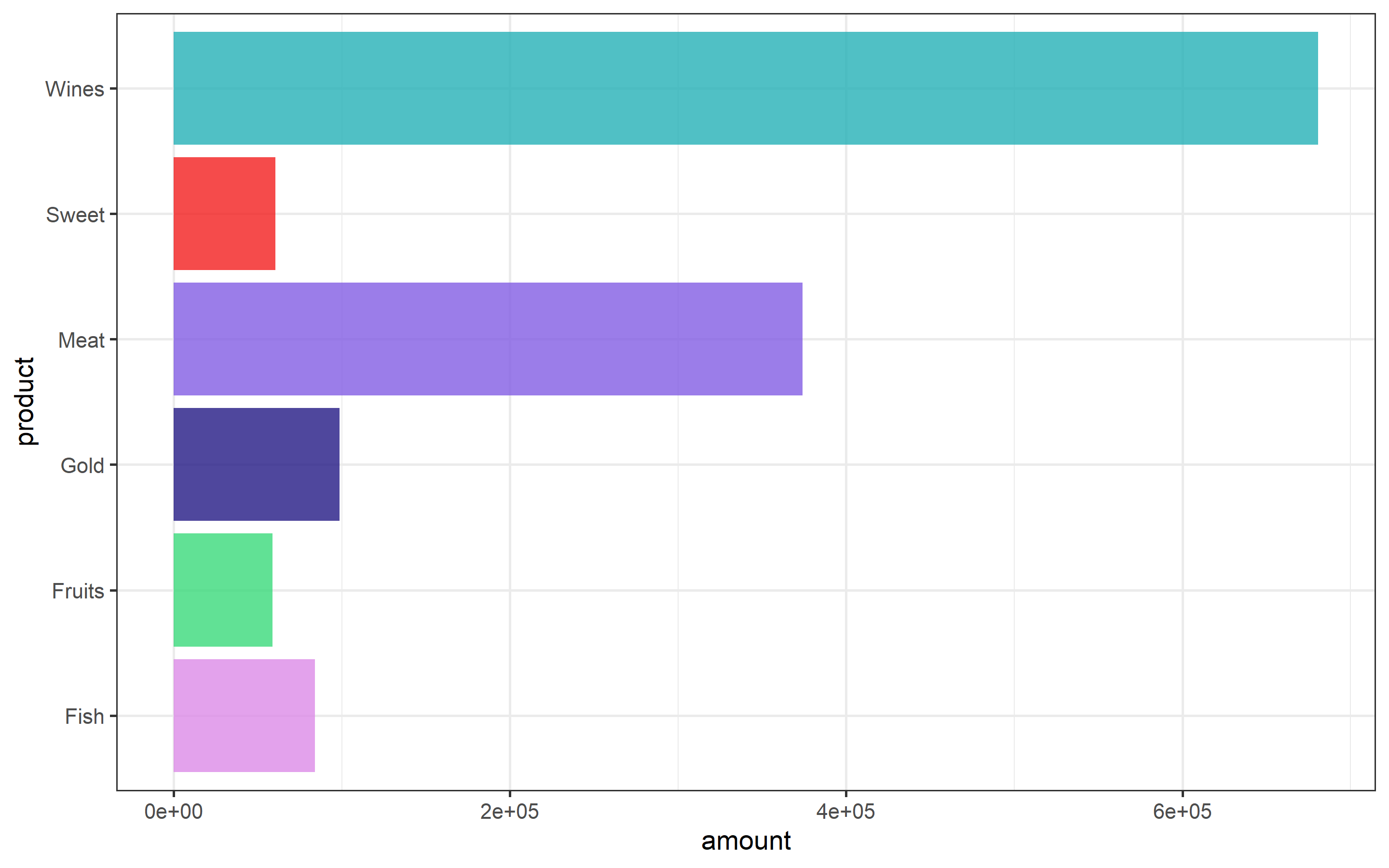 Wines and meat are the channels that are sold the most. On the other hand, sweets and fruits are sold the least. The products that are not performing that well might be put in a bundle/pack to increase the quantity sold.
Section 04: CMO Recommendations
From this analysis, we can conclude that age, kids and teens at home, marketing campaign 1, 3, 5 and the last decrease the number of purchases in store. Whereas, income, campaigns 2 and 4, and products like meat, sweets and gold increase the purchases in store. For total purchases(i.e., the sum of amount spent on all goods) countries have no influence but marketing campaigns 3, 4 and last one affect significantly and positively the total amount spent per costumer in this company. Moreover, costumer who spent more than the average in gold also are more likely to buy in a store. However, married PhD costumer do not buy more fish. In fact, less educated consumers bought more. The 3rd, 4th and last campaign are the most successful ones as we found out before in the regression analysis. Creating bundles of products among those under-performing should increase the amount spent.